Marketing-Mix Modelling

As the World is constantly on the lookout for new technological advancements, advertisement recommendations for sale leads become a necessity for New and Established business to differentiate themselves from their competition.

This project explores Bayesian Mix Market Modelling and report the findings of the created Machine Learning model with the scope of predicting sales and recommending the most appropriate advertisement strategy for sale leads.

Methods

Bayesian inference is a method of assigning a probability distribution to a parameter. These probability distributions express some degree of uncertainty of a value for the parameter. The aim of inference is then no longer to find the “best” single value for the parameters of the model, as in other statistical models. Rather it is to determine the posterior distribution of the parameters. This posterior distribution is determined by a
combination of the likelihood of the data, and prior knowledge of the parameter distribution. The posterior distribution is therefore described by a simple expression of Bayes’ Theorem:

The likelihood is the likelihood distribution of the data. This distribution summarizes the data, by presenting a range of values for the parameters which is accompanied by the likelihood that the current parameter describes the data. The prior distribution is estimated for parameter values before sampling any data. If no prior knowledge is available non-informative estimates, such as a normal distributions, can be used. AdStock is a method of quantifying the effect an advertisement has on demand over time. Adstock is typically dependent on two factors. Firstly, the decay effect of which an advertisements loses impact over time, And secondly, how the demand of a product scales with the amount of advertising typically is not linear. To take this advertisement saturation into account, the adstock must undergo a transformaion. The Adstock value can then be defined recursively as:

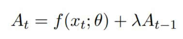
Where At is the adstock to time t, and f(xt; θ) is the transformation function which should be chosen to take ad-saturation into account. This project utilizes a sigmoid transformation of the adstock.
Seasonality traits are periodic fluctuations that can not be attributed to the data given, that might increase or decrease the sales. Examples of seasonality traits include Christmas sales and the like, or weekly occurrences such as the weekend.
The Markov Chain Monte Carlo (MCMC) method is used to approximate the posterior distribution of n parameters through random sampling in a n-dimensional probabilistic space.
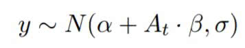
In the project, all of these methods have been combined to predict future sales, and to recommend which channels are the best to advertise on. Through Bayesian inference the likelihood of the data has been calculated as:

Using the MCMC method the approximation of the posterior distribution for each of the parameters have been found. The effect an advertisement channel has on sales can be evaluated by removing said advertisement from the prediction of a model, and noting the effect of this on prediction. The drop in sales compared to the money spent on this channel can then be depicted as an indication of it’s usefulness.
Intuitively it can be induced that if a model still predicts well, even after the data describing the channel has been removed, that this channel has very limited effect on sales. Similarly, if the model drops significantly in sales after removing the advertisement data, said advertisement must have a positive impact on the sales.

Experiments

The dataset consists of daily data points spanning over three years, describing the amount of money that was spent on several different types of advertising, and their respective impressions. The dataset also consists of two external factors, the amount of sunshine, and the currency between EUR and USD.
Using a model which uses all five impression features of the dataset, a Root Mean Squared Error (RMSE) of 36.55 was achieved on unseen data.

Moreover, if the same model is applied to the training set, the model achieves an RMSE of 66.04 2. This result can also be seen in table 1.

Table 1 also shows the scores of different model setups on the entire training dataset. The only parameters which were changed in this experiment was the number of features, and more specifically which ones. The seasonality patterns and prior distributions have been left as in the baseline model.

The results of the method in table 2 showed that when removing TV-ads sales dropped ∼ 57%. Removing radio ads the average sales dropped ∼ 17%. Removing ’ooh’ ads, the sale essentially stayed the same. Removing ’searchppc’ and ’display’ ads in fact increased the sales, by respectively ∼ 3.5% and ∼ 13.5%.

Discussion

To find different seasonality traits, periodic poor predictions were observed. If an inaccuracy in score is consistent in periodic jumps, it is an indication that a seasonality trait is at play, that the model can not describe. These seasonality traits were manually found and implemented in the model, and resulted in a huge increase in prediction scores. An example of such a seasonality traits in the project data is sales on Black Friday. In the data, the sales spike on this particular day, due to the seasonal event. Moreover, a
pattern for each quarter of the year was found. Here the same three months of the year, have somewhat similar tendencies across all three years of the data. These patterns can be seen on figure A.1

The current model is at a stage of good performance. However, improvements to the performance could still be made. The amount of experimentation on hyper parameters have been limited due to time constraints.
However, in table 1 results from testing different combinations of features on the same baseline model can be seen. It can be seen that ’searchppc’, ’ooh’, and ’display’ has the smallest impact on the model when removed. However, working with only the TV and Radio impressions did have a larger impact on the model performance than the first results signaled. The preferred model for this project is therefore the one using
all of the impression features.

According to the established model, it can be deduced that TV-advertisement and radio has the greatest effect on sales. Using Tv-ads, in particular, produces a very large increase in sales. Even though the most money was spent on it (∼7,000,000), the drop in sales compared to money spent when removing TV-ads from prediction is very large. The sales when removing radio-ads did not fall as drastically, also when compared to the amount of money spent (∼ 40% less than tv-ads). Furthermore, it can also be deduced from the model that spending ∼ 3, 000, 000 on ’ooh’ ads could have been money better spent, as it showed to have very little influence on the sales of our model.
As our model shows that money is best spent on TV-ads, the saturation effect of ads is not taken into account. At some point it would be better to spend more money on Radio-ads, when the saturation of TV-ads has become so high that the demand becomes lower per dollar than radio-ads. Finding this point could be an analysis for future work.

Concluding remarks and future work

This project was about Marketing Mix modelling and to predict future sales and recommend optimal channels for advertisement. It was found that spending money on ’Out Of Home (ooh)’ ads was largely a waste of money compared to TV- and radio advertising. This was shown, both by removing the feature completely
from the model and removing it during predictions.
Due to lack of time, the model does not include two variables from the data set: sunshine and US EUR exchange rate. The model therefore has no external factors impacting performance. A good next step would then be to incorporate these variables. Moreover, more work on finding appropriate priors would too be an ideal next step for the project.

A Appendices
A.1 Seasons – Spring, Summer, Autumn, Winter

A.2 Resulting Graph

Figure 2: Predicted values (Blue) Compared to true values (Red). Y-axis depicts the sale to time on X-axis